1. From Sensor Signal to Inference Input:

Once a TinyML model is integrated into an embedded system, runtime behavior follows a simple and repeatable pattern. The device continuously or periodically collects sensor data, prepares it in a predefined format, and runs inference to obtain a result. This process is deterministic and does not change once the firmware is deployed.

In a vibration monitoring system, this begins with sampling raw acceleration data at a fixed rate. Samples are collected into a fixed-size buffer whose layout and size are defined during model design. These parameters remain constant at runtime to ensure predictable memory usage and execution behavior.

Before inference, the raw data may undergo basic preprocessing such as windowing, normalization, or simple feature extraction. These operations are typically lightweight and are chosen to match the assumptions made during model training. Their purpose is not to interpret the signal, but to present it in a form the model expects.

From an embedded systems perspective, this stage closely resembles a traditional signal-processing pipeline. Data acquisition, buffering, and preprocessing are performed deterministically and use statically allocated memory. The difference lies in the final step: instead of passing the prepared data to hand-written decision logic, the system hands it to a TinyML inference engine that produces an output based on learned patterns.

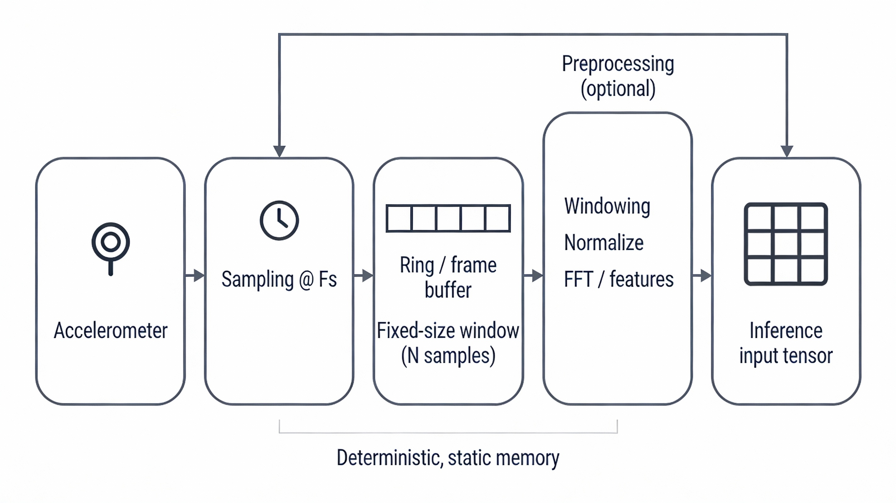
Fig. 1. Input data flow from vibration sensor to a fixed-size inference buffer.

2. Model Representation in Embedded Memory:

Once the input buffer is ready, inference operates on a prebuilt model stored in non-volatile memory. The model consists of a set of weights and a description of the operations required to process the input data. These weights are generated during offline training and are never modified at runtime.

In the vibration monitoring system, the model is linked directly into the firmware image, typically as a binary data structure. There is no dynamic loading, parsing, or modification of the model while the system is running. This approach avoids reliance on file systems and dynamic memory allocation, keeping runtime behavior predictable.

From the system's point of view, the model is simply read-only data stored in flash. Accessing it during inference is no different from accessing constant lookup tables or calibration data used elsewhere in the application.

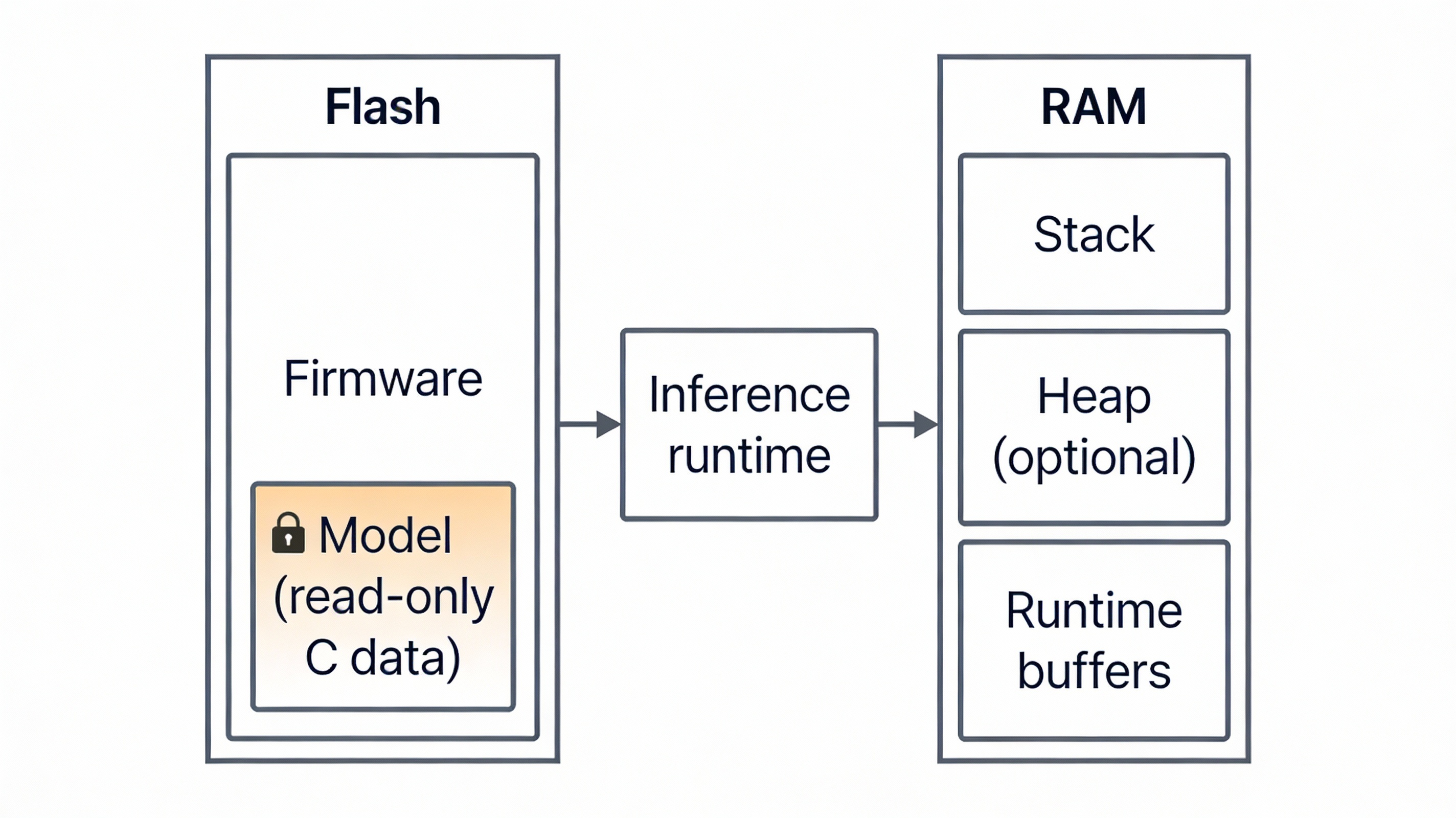
Fig. 2. TinyML model stored as read-only data in flash memory and accessed by the inference runtime during execution.

3. Inference Execution Flow:

When inference begins, the runtime executes a fixed sequence of operations defined by the model. These operations are typically small numerical kernels that process the input buffer and intermediate results layer by layer. The execution order is static and known at build time.

For the vibration monitoring example, every inference follows the same execution path regardless of the input signal. There are no data-dependent branches and no dynamic control flow. This makes inference deterministic and well suited to real-time embedded systems.

The runtime processes the input buffer, applies the model operations, and produces an output tensor. From a scheduling perspective, inference behaves like a bounded computation whose execution time can be measured and budgeted alongside other tasks.

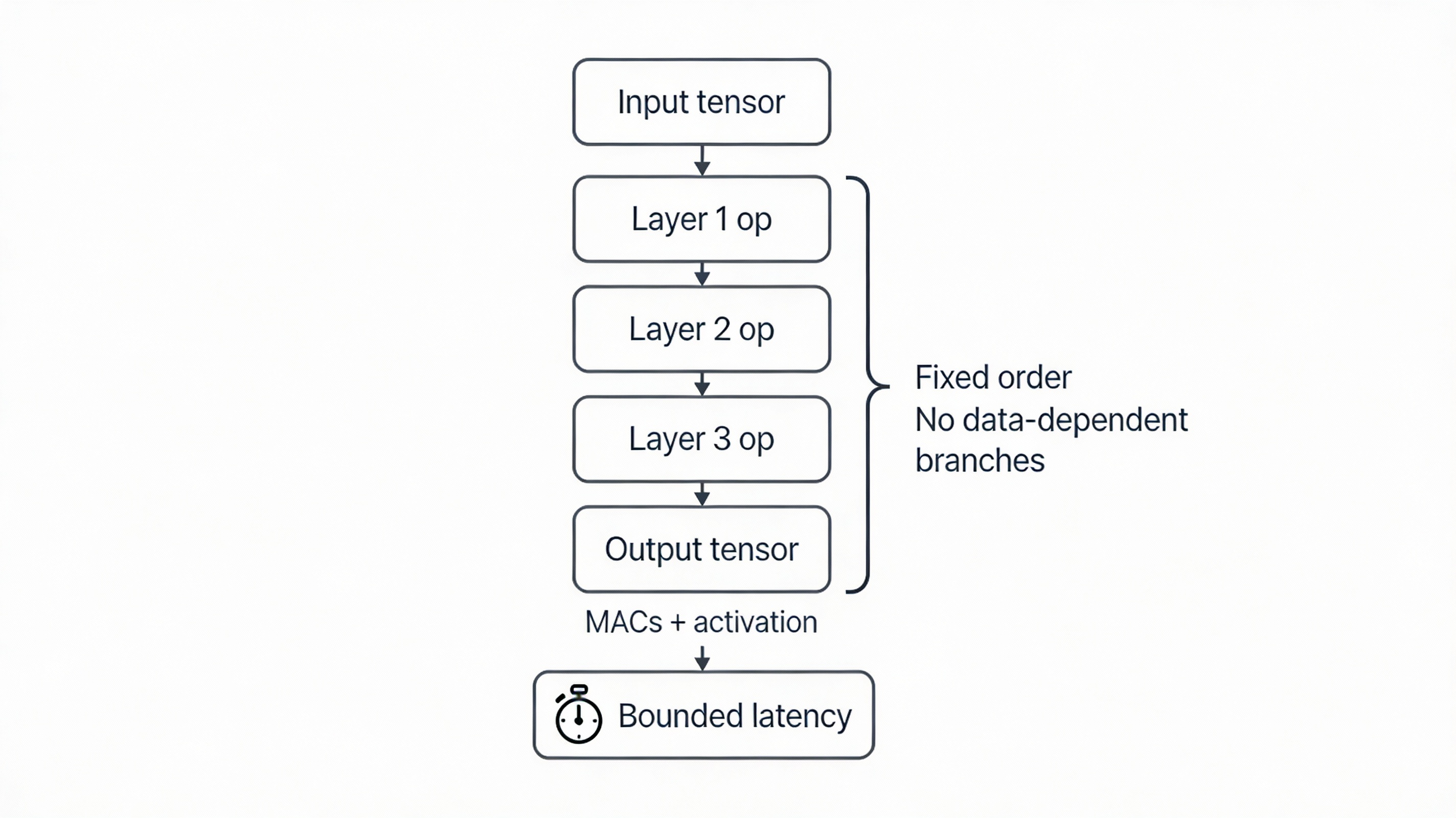
Fig. 3. Fixed execution flow of a TinyML inference

4. Interpreting the Output:

Once inference completes, the model produces an output that represents the result of pattern recognition. This output is not a direct decision, but a numerical indication of confidence or likelihood.

In the vibration example, the output may indicate how closely the current signal matches patterns associated with abnormal behavior. Application code must interpret this value and decide how to act on it. This often involves applying thresholds, time-based filtering, or state logic to avoid reacting to transient conditions.

At this stage, TinyML integrates back into traditional embedded design. The model output becomes just another input to the system's control logic, alongside timers, counters, and other sensor data.

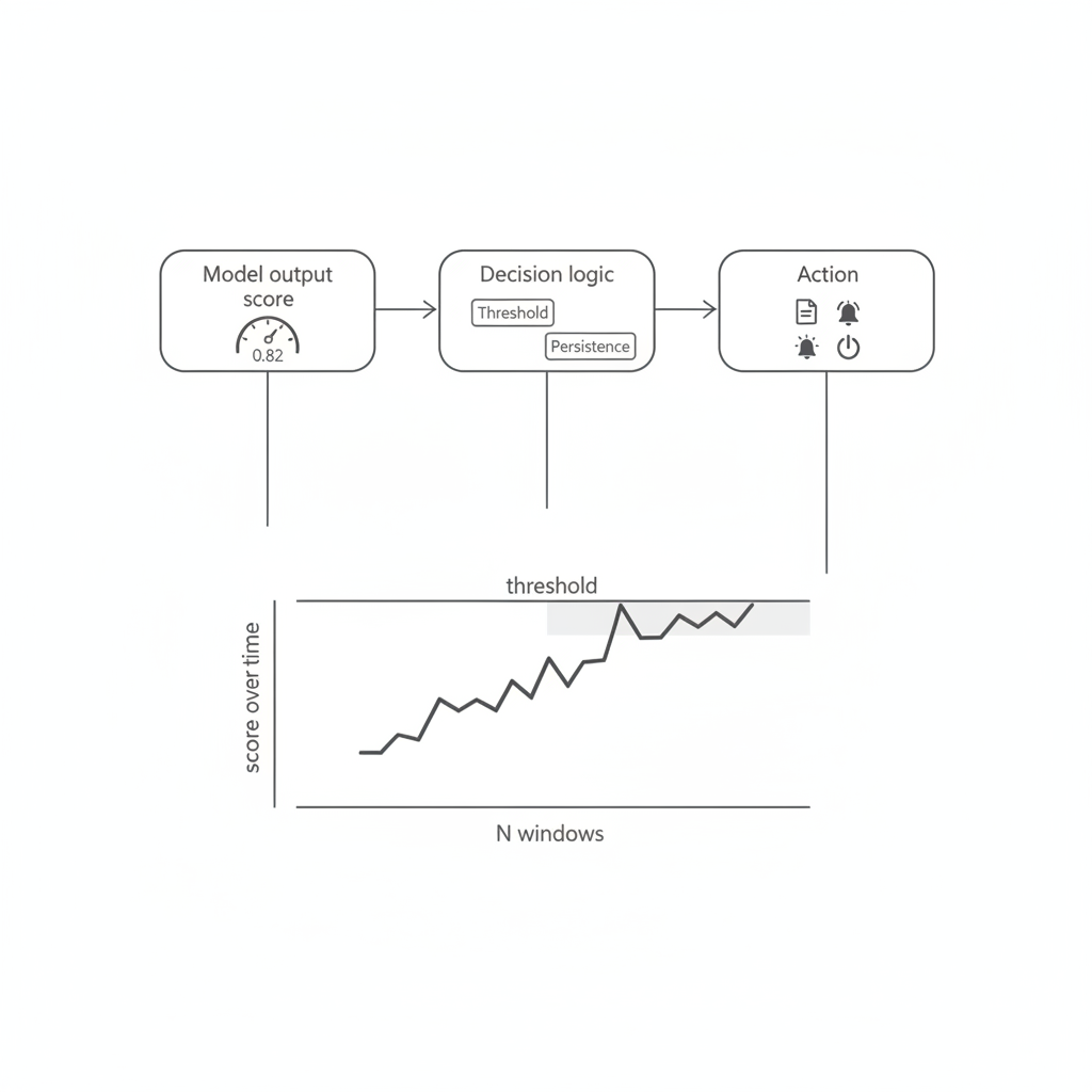
Fig. 4. Integration of TinyML inference output into application decision logic.

5. Determinism, Timing, Power, and Hardware Support:

Although TinyML uses machine learning techniques, inference on an embedded device behaves deterministically at runtime. Given the same input buffer, the model follows the same execution path and produces the same output. This predictability is essential for real-time and low-power systems, where execution time and behavior must be bounded and repeatable.

Inference timing must be considered alongside sensor sampling, communication, and control tasks. In a vibration monitoring system, inference may run periodically or be triggered by specific events. In either case, its execution time must fit within the system's scheduling constraints and coexist cleanly with other real-time workloads.

Power consumption is closely tied to these timing decisions. Running inference too frequently increases energy usage, while running it too infrequently may reduce detection reliability. Balancing responsiveness and power efficiency is therefore a system-level design choice rather than a property of the model itself.

These practical constraints have directly influenced modern system-on-chip designs. TinyML is no longer treated as an experimental workload layered on top of general-purpose hardware, but as a concrete use case that shapes how compute units, memory hierarchies, and data movement are organized inside the SoC.

As a result, many modern microcontrollers and low-power SoCs integrate DSP extensions, SIMD instructions, or lightweight neural acceleration blocks. These features are well matched to the computational patterns used in TinyML inference, such as convolution, filtering, and vector arithmetic. Supporting these operations directly in hardware reduces inference latency and energy consumption without changing the embedded programming model.

The motivation behind this hardware investment is practical. Many embedded applications require continuous local analysis of sensor data, including vibration, audio, and motion signals. Offloading this processing to the cloud introduces latency, bandwidth usage, and power costs that are incompatible with always-on systems. Executing inference directly on the SoC enables fast response times, predictable timing, and efficient energy usage within tight constraints.

Conclusion:

A TinyML inference is best understood as a structured embedded workload rather than a black-box machine learning operation. Input data is collected into fixed buffers, processed through a static sequence of operations, and converted into an output that feeds existing application logic. Memory usage, timing, and determinism remain central concerns.