1. Introduction

Performance analysis has always been one of the toughest challenges in computer science. At its heart, it’s about figuring out how programs actually use the CPU, memory, and I/O while they run. The rule of thumb is simple: if you can’t measure how your system behaves, you can’t really make it faster.

But in practice, that’s easier said than done.

Picture a familiar situation: an application runs flawlessly during development, but once it’s deployed under real workloads, it starts slowing to a crawl. CPU usage spikes, response times stretch out, and the system suddenly feels unresponsive. The worst part? There’s no clear sign of what’s wrong. Without the right tools, developers are left guessing whether the bottleneck comes from their own code, a third-party library, the kernel, or even the hardware itself.

This disconnect between what you see and what’s actually happening is where profiling comes in. On Linux, a wide range of profiling and tracing tools exist to make the invisible visible. From simple counters that track CPU usage to detailed sampling of functions and system calls, they give developers the insight they need to turn vague performance problems into clear, actionable fixes

2. What is Profiling?

Profiling is the practice of watching a program run and recording how it uses system resources over time. In the simplest terms, it’s about answering questions like: How much CPU does this program really consume? Where does it spend most of its time? Is it waiting on memory, disk, or the network? By collecting this kind of information, developers gain a clear picture of the program’s behavior instead of relying on guesswork.

It’s important to distinguish profiling from tracing. Profiling usually works by taking samples at regular intervals, building a statistical view of where the program spends its cycles. Tracing, on the other hand, records individual events—every system call, every function entry, every context switch. Tracing gives you fine-grained details but produces a lot of data, while profiling provides a higher-level overview that’s easier to digest.

Both approaches are valuable, but when the goal is optimization, profiling is often the first step. Without it, developers risk “optimizing” the wrong parts of the code—spending days rewriting a function that only accounts for 1% of execution time, while ignoring the real bottleneck that eats up 80%. In other words, profiling ensures that effort is focused where it truly matters.

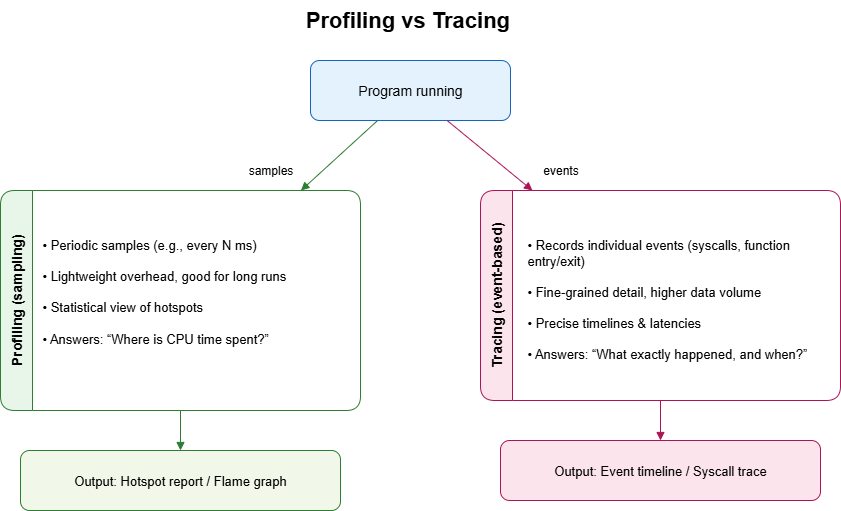
Fig. 1 – Profiling vs. tracing approaches

3. Common Tools for Linux Profiling

Linux provides a rich toolbox for understanding performance. Each tool has a different focus, from quick measurements to deep dives into kernel events. The trick is to pick the right one for the question you’re asking.

Basic Measurement Tools

• time

The simplest profiler. Measures how long a command takes, along with user and system CPU time.

Perfect for quick checks.

• top / htop

Real-time monitors that show which processes consume the most resources.

- htop adds color, interactivity, and per-core CPU views.

- Useful for spotting runaway tasks.

Performance Counters

• perf

The Swiss army knife of Linux profiling.

- Measures CPU cycles, cache misses, and function hotspots.

- Often the first tool serious developers reach for.

• pidstat

Provides per-process statistics over time.

- Shows CPU, memory, and I/O activity.

- Ideal for profiling long-running workloads.

Tracing Tools

• strace

Traces every system call a program makes.

Great for finding bottlenecks in file I/O, networking, or unexpected syscalls.

• ftrace

A kernel-level tracer.

- Digs into function calls inside the Linux kernel.

• eBPF tools (bcc, bpftrace)

The modern powerhouse.

- Attach tiny programs to kernel events.

- Collect metrics and build custom profilers without rebooting or recompiling.

- Flexible, powerful, and production-ready.

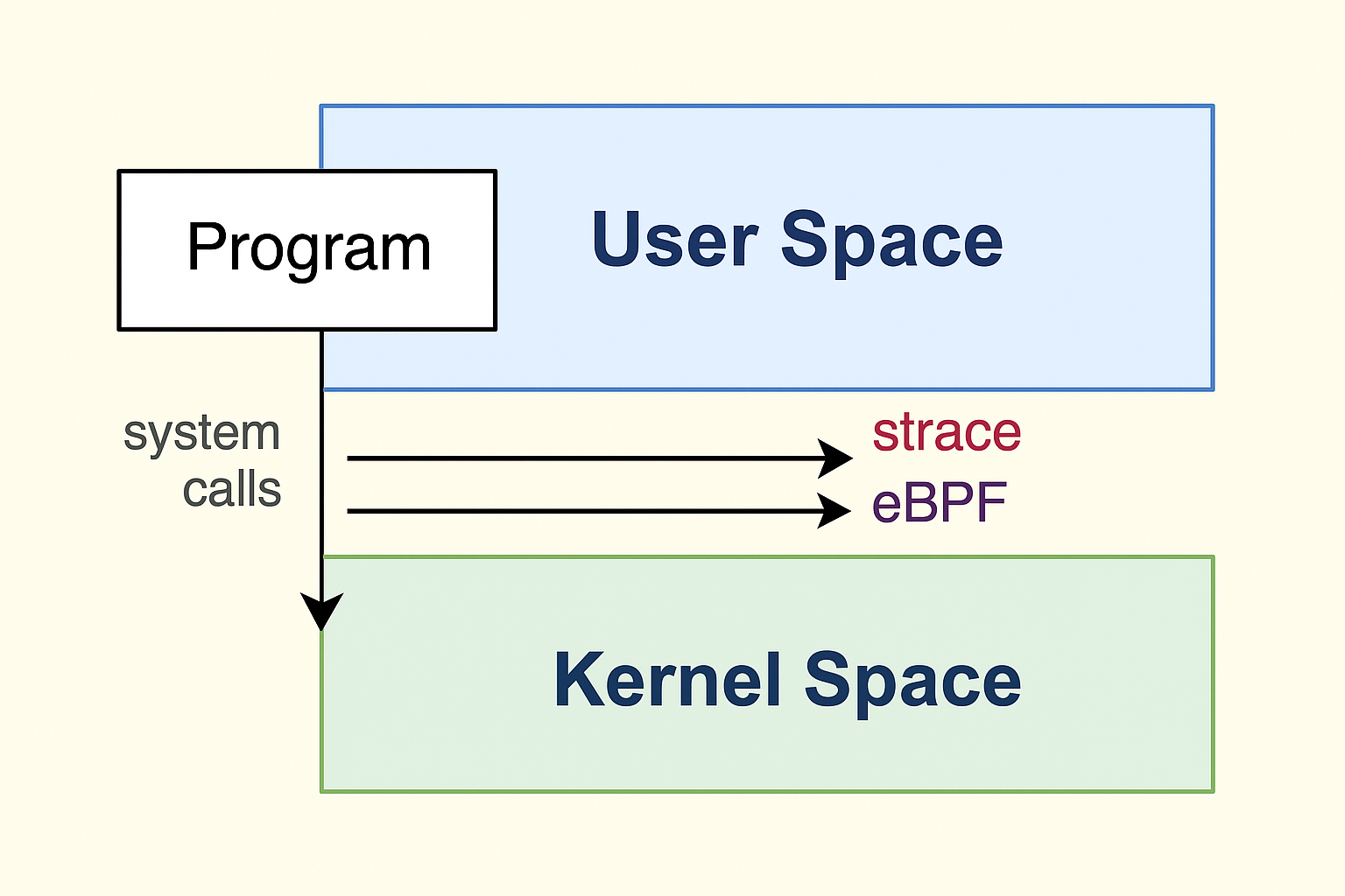
Fig. 2 – User space and kernel space with system call tracing

Memory and I/O profilers

• valgrind

Heavy but precise.

- Catches memory leaks and invalid accesses.

- Can simulate cache usage.

- Ideal for debugging tricky bugs, though it slows programs down.

• iostat

Focuses on disk throughput and latency.

- Reveals when a program spends more time waiting for I/O than crunching CPU.

Each of these tools looks at the system through a different lens. Together, they give developers a full picture: whether the slowdown comes from CPU-bound code, excessive syscalls, memory leaks, or storage bottlenecks.

4. Practical Examples of Profiling

Theory is useful, but the real value of profiling comes from trying it on actual programs. Let’s look at two simple but instructive examples:

Example 1: Profiling a CPU-Bound Loop

A classic case is a program that spends most of its time crunching numbers.

#include <stdio.h>
int main()
{
    long sum = 0;
    for (long i = 0; i < 1e9; i++) 
    {
        sum += i;
    }
    printf("%ld\n", sum);
    return 0;
}

The program is first compiled without optimizations:

gcc -O0 loop.c -o loop

When executed with the time command, the results show a long runtime, with nearly all the time spent in user space.

time ./loop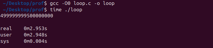

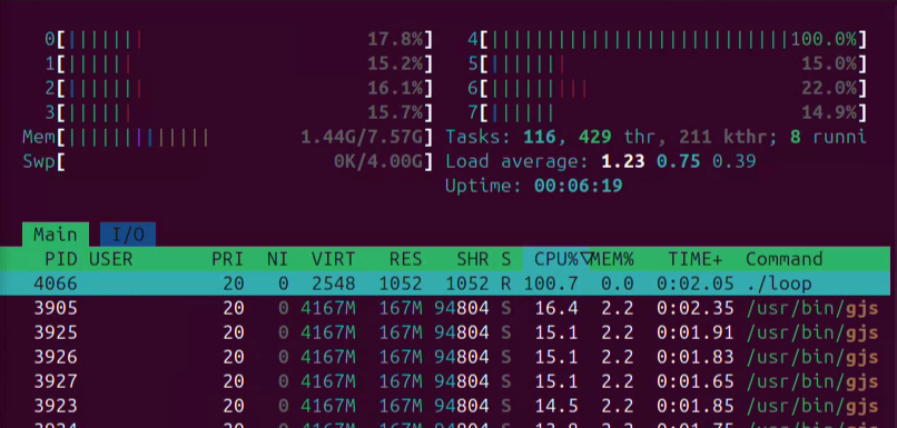
While the program is running, system monitoring with htop reveals a single CPU core at 100% utilization, confirming that the workload is entirely CPU-bound.

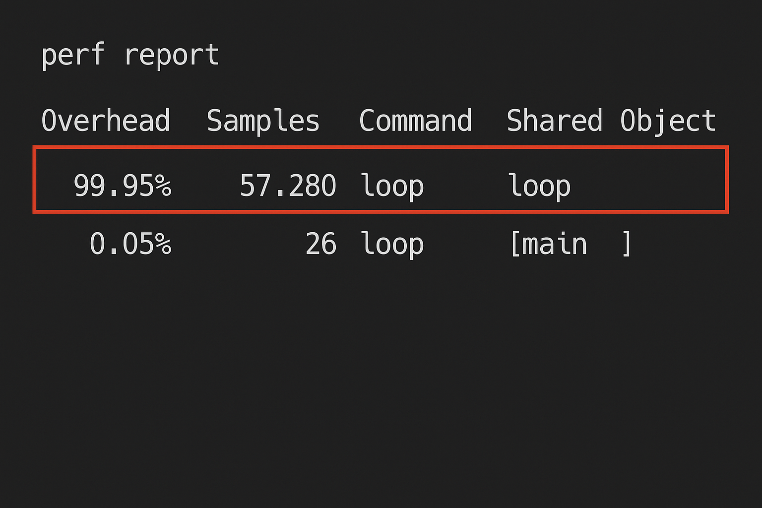
Using perf gives a clear view of execution hotspots.

First, record the program’s activity:

perf record ./loop

Then generate the report:

perf report

The report shows that almost all the CPU cycles are consumed inside the main function, which contains the large loop.

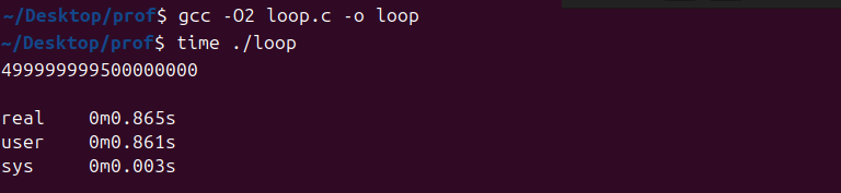
Recompiling the program with optimizations enabled produces significant change:

gcc -O2 loop.c -o loop
time ./loop

Execution time drops significantly, and profiling tools report minimal activity, since the compiler optimizes away most of the loop.

This example highlights two key insights: profiling makes it clear where the CPU time is spent, and it also provides measurable proof of the impact of optimizations.

Example 2: Profiling an I/O-Bound Program

Not all performance bottlenecks come from CPU-intensive loops. Many real-world applications spend most of their time waiting on input and output. A classic case is traversing a large directory tree on disk.

Consider the following command:

ls -R /usr

This command recursively lists the contents of the /usr directory. On most systems, it generates a very large output and touches thousands of files and subdirectories. The workload is limited not by raw CPU power, but by the speed of file system operations.

To see this, run the same command under strace with the -c option, which summarizes all system calls:

strace -c ls -R /usr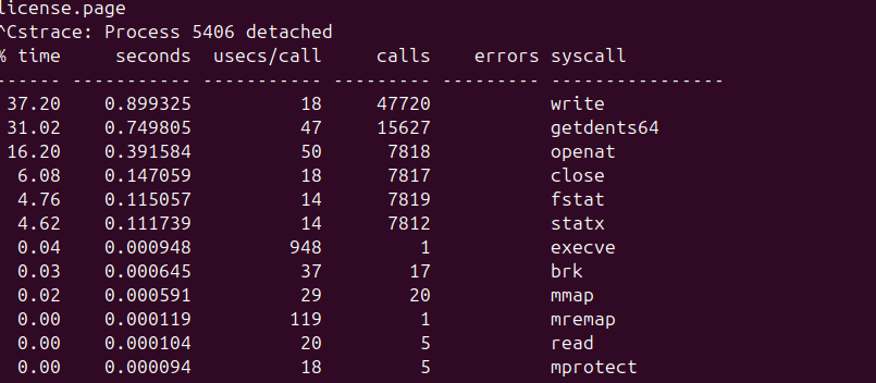

The results clearly show that the program spends most of its time performing calls like getdents (reading directory entries) and stat (checking file metadata). Instead of consuming CPU cycles in a tight loop, the program is repeatedly asking the kernel for file system information.

5. Conclusion

Profiling is not about guessing—it’s about seeing. By combining the right tools, developers can move past vague symptoms and uncover the real reasons behind slowdowns. Whether the issue lies in CPU loops, system calls, or disk I/O, Linux offers everything needed to shine a light on performance bottlenecks. Once the data is visible, optimization stops being guesswork and becomes engineering.